Building a Spatial Index Supporting Range Query using Space Filling Hilbert Curve
By Forest Johnson On
I was feeling burnt out this month, not motivated to work on my serious-bizznezz projects like greenhouse.
Later, reflecting on how I was feeling, I realized:
I haven't worked on a project just for fun, to see what I can build for its own sake, not as a means to an end since before I started working "professionally" when I was like.. 14
I'm sure that's hubris; but after "letting myself go", getting excited about building something for fun & subsequently hyperfocusing and going on random project tangents for a week, I can say I definitely missed this, whatever it is.
Anyways, today's topic returns my blog to its "sequential read" namesake, and I can't think of a more beautiful way to do it. I can't wait to write about it, but first, I have to talk about what a spatial index is & why anyone would need such a thing.
And before I talk about spatial indexes, I probably need to talk about files.

Yes, files. Those things I leave on my desktop, piling up in an ever expanding array stretching across both my screens, until both screens are full and my linux desktop starts bugging out, forcing me to find other ways to sift through them.
Files are THE interface for storage on computers. If you've never written a file byte-by-byte yourself in a program, you might not be intimately familiar with the underlying interface, but files are treated like streams of bytes, one coming after another. This linearity probably harkens all the way back to spools of tape that were used with early computers,

or even the cosmic masses of theoretical paper tape associated with Turing Machines.
This linearity of files is built into just about every single storage API and storage hardware device under the sun. While some things may be slowly changing in the storage world (private browsing mode to evade paywall), this idea of streaming a linear sequence of bytes from a storage device probably isn't going anywhere soon. It's a really good idea; it works very well for just about everything.
Database indexes like Log Structured Merge Trees employ clever sleight of hand, carefully organizing and layering many of these streams on top of one-another (plus RAM) to provide an incredibly fast, stable & scalable storage engine. The LSM idea sparked all of the excitement about "noSql" or "key/value" databases like Apache Cassandra and leveldb 10 years ago because it was so simple & easy to scale horizontally on a "cluster" of multiple database servers.
This breed of storage engine typically offers an API that looks something like this:
put(key,value) -> nullget(key) -> valuerangeQuery(startKey, endKey) -> iterator<[key,value]>
In other words, they allow us to do three different things, either:
-
Assign a value to a given key, like "The name printed on mail box number 55 (
key) is now 'Jeremy' (value)." -
Retrieve the current value (or
nullif no value was specified) for the given key, like "What name is printed on mailbox number 55? Oh, it's Jeremy." -
Scan the database for any keys that fall between a given range, like "Within the row of mail boxes from 50 to 60, are there any that are claimed? Oh, I see one, number 55. It was claimed by Jeremy. Oh, here's another one, number 58. It was claimed by Trisha."
Importantly, the act of scanning or rangeQuery-ing directly maps to the way the computer reads one byte after another from a file stream. A "SequentialRead" if you will 😏
This means that the data for the keys and values must be laid out in sorted order within the files. LSM indexes have a really clever way of doing this, and there are others, like B+ trees, but the details of how that happens is out of scope for this post.
This scheme of building everything out of put, get, and rangeQuery is more powerful and flexible than it might seem, but it can get frustrating sometimes. What if I'm not storing and looking up up mailbox numbers, email addresses, events that happened on Friday, or objects in categories? What if I want to look up all restaurants within 1 mile of my current location, or all known stars visible within a certain angle relative to the Crab Nebula?
It may not be immediately obvious, but there's a huge problem here. When I'm storing restaurants or astronomical entities in my index, I'm going to want to to use their positions as the first, most significant part of the key, because that's what folks are going to want to query the data based on.
While these fast key/value storage engines often come wrapped with plenty of convenient conversion logic built in by the time they reach your desk, underneath they are working with bytes. The keys and values are all just strings of bytes, or long binary numbers, and they will be sorted that way.
So I'm presented with a conundrum:
Say that my object has position
[x,y]. How do I convert that to a key? Should I place thexbytes first, and then theybytes? Or the other way around?
Unfortunately, they are both the wrong answer. We build database indexes because we want to house data which is much larger than the amount that one computer can load at one time -- database indexes are an absolute must when the universe of your data is much larger than a single user's view of it at any given time. So any time you're looking at a result from a database query, it's often the tip of the iceberg. There's potentially unlimited amounts of data you can't see outside of the scope of your query.
Say we try to perform a rangeQuery against an index of keys that are laid out like [y,x], and we want to query the rectangle spanning from [4,1] to [5,5] like so:
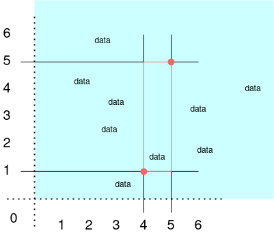
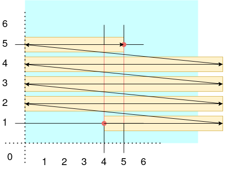
If we naively rangeQuery from [4,1] to [5,5], we'll end up crashing directly into that "potentially unlimited amounts of data" iceberg: the query will have to scan through all data on rows 2 through 4, and half of rows 1 and 5:
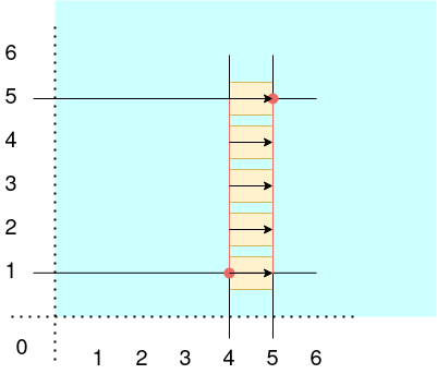
Of course, after your users come back and complain that the system doesn't work, query requests are timing out, you update the code: whenever there is a query that spans multiple rows, each row will get its own rangeQuery:
rangeQuery([4,1],[5,1])rangeQuery([4,2],[5,2])rangeQuery([4,3],[5,3])rangeQuery([4,4],[5,4])rangeQuery([4,5],[5,5])
There! We did it! Crisis averted!... For now.
The problem is, eventually Queries Georg is going to start using your application and run a query that spans a million rows, triggering a million file i/o operations. So this isn't going to work very well either.
This is why we need spatial indexes (some people say "Geospatial"). A proper spatial index can handle queries for "all things within this rectangle" or "all things within a certain distance of a point" much more gracefully, without seeking to a million different places within the database file, or even worse, trying to read the entire file.
However, due to files and storage devices linear natures, we have to come up with clever ways of achieving this. Particularly, I'm interested in ways that I can get a real spatial index without having to throw away my current storage engine and its associated database files / code. Typically, spatial indexes are a "fancy", rare, or hard to find feature in the database world, so it would be nice if we could build a spatial index out of the simple put, get, and rangeQuery primitives that every key/value storage engine (and every relational SQL-ish database) offers.
This is where that "math" stuff they kept trying to teach you to hate when you were a kid really "turns over a new leaf" and becomes awesome. It turns out that there is a class of mathematical constructs called space filling curves which are uniquely suited to this task. A space-filling-curve is a single wiggly line that noodles its way around a two or three dimensional space, never intersecting itself, never running over itself, and covering the entire space. Typically, they are also fractals, meaning that they can always become finer and finer, with infinitely more and more intricate detail. As the (apparently rigorously defined & proven) story goes, at the "limit" as the amount of detail approaches infinity, length and area become the same thing and the curve actually fills the entire space.

Why does this help us? Well, because it allows us to transform a two dimensional space [x,y] into a one-dimensional space [d], where d represents the distance traveled along the curve. We can also transform the opposite direction, from any given distance d along to curve to a cartesian point [x,y].
You might start to see where I'm going with this already, we're going to end up using d as the key in the database index instead of x,y or y,x.
But before going on, I definitely recommend checking out Grant Sanderson (3blue1brown)'s excellent video about the Hilbert curve and other space filling curves.
I decided to base my code on this particular Hilbert Curve implementation from google because it looked simple and fast, and supported both the 2D -> 1D & 1D -> 2D transformations.
I set out to create my first spatial index. First, I followed a Golang OpenGL boilerplate tutorial to get a graphical application running where I could draw pixels and see them show up on screen. Making a whole OpenGL scene from scratch is probably overkill for what I was doing, but I was having trouble finding any alternatives, and it ended up being not so bad, as I recognized a lot of the 3D graphics API stuff from back in my Unity3D days.
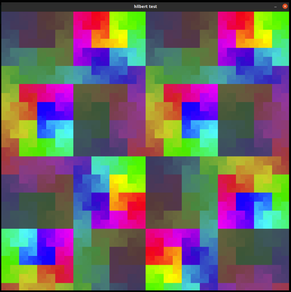
Once I got my textured plane rendering to the screen via OpenGL, I colored the texture based on the 2D -> 1D transformation function. For each pixel in the image I would calculate its associated distance along the curve based on the pixel's [x,y] position, and then create a color based on that distance. In this image, I had configured it to spin the color's hue around the color wheel as the distance increased, and to also slowly oscilate the saturation and brigtness up and down based on the distance using a Sine function.
After that, I began experimenting with ways to map a range of pixels (a rectangle defined by a point and width+height) to a segment on the curve defined by a starting distance and ending distance.
I figured out pretty quickly that I'm not going to be able convert every rectangle to a single curve segment. Just think about it, the color and the saturation in the image above are based on the distance along the curve -- so anywhere that you see a high contrast between two different colors right next to each-other represent areas of the curve having close physical [x,y] proximity, but being vastly separated in terms of the distance along the curve.
However, I was fairly sure I could get it down to handful of curve segments, like 2 or 3, and never more than that. When designing algorithms, these are the kind of problems that you prefer to have. Multiplying the amount of time my algorithm takes to run by a constant factor like 2 or 3 isn't going to cause problems in the grand scheme of things. It's worlds better than trying to run a separate rangeQuery for every single row.
At first, I tried sampling all the curve points along the edges of the rectangle to obtain thier corresponding distances along the curve, then sorting the list of distances and attempting to determine contiguous sections based on the data in the sorted list.
Finally, the code would come up with some curve segments it thought would cover the rectangle based on the data in the sorted list. Then the next time OpenGL prompted me to re-draw the texture, I would highlight all the pixels that fell within those curve segments.
Sometimes it worked,

sometimes it didn't.

I think I would sometimes get the empty rectangles because my code had no way to tell the difference between "these two points are distant because the curve goes far outside the rectangle" versus "these two points are distant because the curve between them wiggles around a lot inside the rectangle."
Eventually I gave up and simply had the code sample the entire area of the rectangle, and this was when I had my first taste of real success:
The query rectangle is shown in white, and the colorful flickering areas around it represent the segments of the curve that the rectangle is being mapped to.
The numbers printing out on the bottom document how many individual curve segments the rectangle has been mapped to.
The black bar with flickering white lines on the top is a number line representing the entire curve. The flickering white lines show the specific areas of the curve which are directly intersecting the rectangle. The left edge of the black bar represts the beginning of the curve, and the right edge the end of the curve.
Now the problem was that sampling the entire rectangle gets slow quickly as the rectangle gets larger -- the number of samples is squared, representing the area of the rectangle. As you can see in the video, even with my relatively small 512x512 curve, the larger rectangle sizes caused the app to slow down a lot.
This stumped me for a long time, but I eventually figured out how to carefully scale down the rectangle and the curve itself to a lower resolution until the rectangle was small enough that sampling its area wouldn't cause the CPU to break a sweat. Remember how the Hilbert curve is a fractal? And not only that, like Grant showed, it's continuous from order n to order n+1, meaning that scaling it down to a smaller resolution won't move things around much; in terms of percentages, both the 2D -> 1D and 1D -> 2D transformations will look almost identical. After fixing a few bugs, it was "scrolling like butta" before my very eyes, even with the curve length cranked all the way up to math.MaxInt64!
In the second video, I added additional printout documenting how much "extra" un-needed space is being queried as well as how many curve segments were created. I also changed the behaviour of the white bars on the curve-numberline at the top; now they show the entire selected curve segments, not just the areas of the curve intersected by the rectangle.
One of my favorite things about this project: There is a tweakable parameter iopsCostParam controlling when the code decides to split up a particularly wasteful curve segment into two less-wasteful segments.
// iopsCostParam allows you to adjust a tradeoff between wasted I/O bandwidth and # of individual I/O operations.
// I think 1.0 is actually a very reasonable value to use for SSD & HDD
// (waste ~50% of bandwidth, save a lot of unneccessary I/O operations)
// if you have an extremely fast NVME SSD with a good driver, you might try 0.5 or 0.1, but I doubt it will make it any faster.
// 2 is probably way too much for any modern disk to benefit from, unless your data is VERY sparse
Length and area are the same thing for this curve, so we can compare them equivalently in the code. The iopsCostParam is used as a threshold ratio between the length/area of a "wasted" section of the curve and the area of the query rectangle itself:
...
distance := curvePoints[i] - curvePoints[i-1]
if float32(distance) > float32(width*height) * iopsCostParam {
    ...
}
...
Benchmarks
The benchmarks are part of the demo repository.
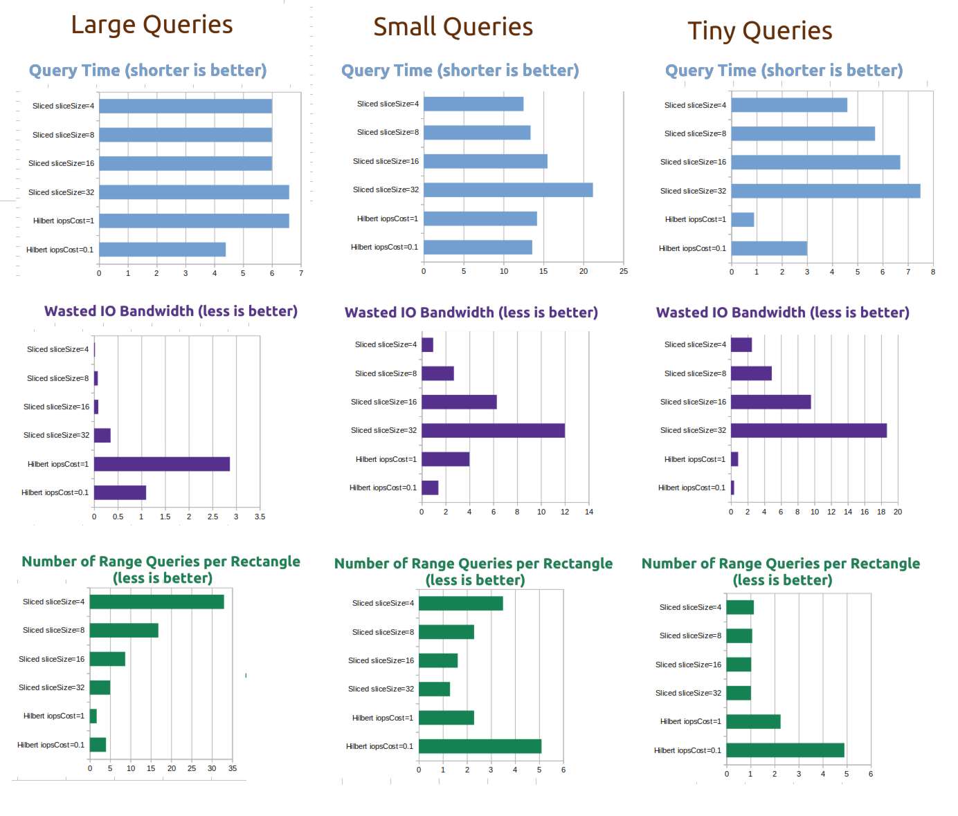
I benchmarked the spatial index against a tuned version of the "One range query for every row in the rectangle" approach I talked about earlier, which I am calling the Sliced index, with various slice sizes.
For a test dataset, I used goleveldb to store approximately 1 million keys, each with a 4-kilobyte random value, with key density determined by the brightness of each pixel on this map:
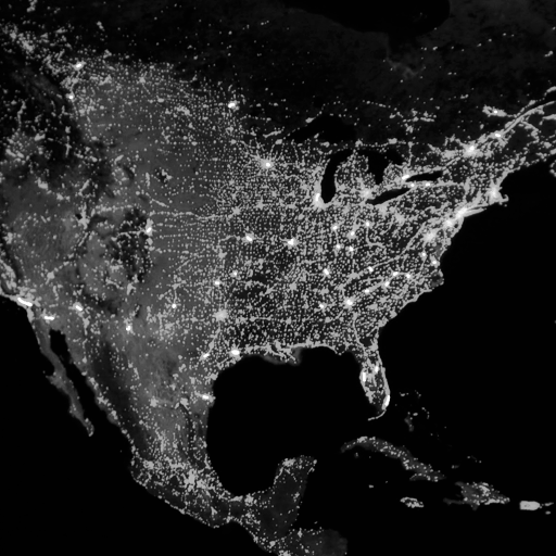
With a 64-bit Hilbert Curve, the keys were indexed with a corresponding real-world resolution of about a milimeter. For a 32-bit curve, the resolution would be about 200 meters.
During the benchmarks, each database index was approximately 3.5GB in size, and the test application was consuming about 30MB of memory. The benchmarks were performed on a laptop with a 8th gen Intel Core i7 CPU and an NVME M.2 SSD hosting the database files.
I believe that my theory was correct; the Hilbert Curve index is not always the fastest, but it's definitely the most predictable in terms of its IOPS and bandwidth demands, and I think that's important.
The other benefit being that the tweakable parameter for the Hilbert Curve range query happens at query time, while the tweakable parameter for the sliced index happens at indexing time -- so with the sliced approach, you can't tune it without re-indexing all your data!
check out the source code on my git server or on GitHub.
Implementation example
See writing keys and querying an area.
Note regarding sillyHilbertOptimizationOffset: The hilbert curve has some rough edges around the center of the curve plane at [0,0], so you will hit worse-case performance (about 3x slower than best case) around there. In my app I simply offset the universe a bit to avoid this.
If your database doesn't support arbitrary byte arrays as keys and values, you can simply convert the byte arrays to strings, as long as the sort order is preserved.
Interface
The interface is simple enough, I think it would be easy enough to use and integrate on top of any key/value database or relational database like SQLite or Postgres:
NewSpatialIndex2D
// This is the only way to create an instance of SpatialIndex2D. integerBits must be 32 or 64.
// To use the int size of whatever processor you happen to be running on, like what golang itself does
// with the `int` type, you may simply pass in `bits.UintSize`.
NewSpatialIndex2D(integerBits int) (*SpatialIndex2D, error) { ... }
SpatialIndex2D.GetValidInputRange
// returns the minimum and maximum values for x and y coordinates passed into the index.
// 64-bit SpatialIndex2D: -1073741823, 1073741823
// 32-bit SpatialIndex2D: -16383, 16383
(index *SpatialIndex2D) GetValidInputRange() (int, int) { ... }
SpatialIndex2D.GetOutputRange
// returns two byte slices of length 8, one representing the smallest key in the index
// and the other representing the largest possible key in the index
// returns (as hex) 0000000000000000, 4000000000000000
// 32-bit SpatialIndex2Ds always leave the last 4 bytes blank.
(index *SpatialIndex2D) GetOutputRange() ([]byte, []byte) { ... }
SpatialIndex2D.GetIndexedPoint
// Returns a slice of 8 bytes which can be used as a key in a database index,
// to be spatial-range-queried by RectangleToIndexedRanges
(index *SpatialIndex2D) GetIndexedPoint(x int, y int) ([]byte, error) { ... }
SpatialIndex2D.GetPositionFromIndexedPoint
// inverse of GetIndexedPoint. Return [x,y] position from an 8-byte spatial index key
(index *SpatialIndex2D) GetPositionFromIndexedPoint(indexedPoint []byte) (int, int, error) { ... }
SpatialIndex2D.RectangleToIndexedRanges
// Returns a slice of 1 or more byte ranges (typically 1-4).
// The union of the results of database range queries over these ranges will contain AT LEAST
// all GetIndexedPoint(x,y) keys present within the rectangle defined by [x,y,width,height].
//
// The results will probably also contain records outside the rectangle, it's up to you to filter them out.
//
// iopsCostParam allows you to adjust a tradeoff between wasted I/O bandwidth and # of individual I/O operations.
// I think 1.0 is actually a very reasonable value to use for SSD & HDD
// (waste ~50% of bandwidth, save a lot of unneccessary I/O operations)
// if you have an extremely fast NVME SSD with a good driver, you might try 0.5 or 0.1, but I doubt it will make it any faster.
// 2 is probably way too much for any modern disk to benefit from, unless your data is VERY sparse
(index *SpatialIndex2D) RectangleToIndexedRanges(x, y, width, height int, iopsCostParam float32) ([]ByteRange, error) { ... }
ByteRange
// Use this with a range query on a database index.
type ByteRange struct {
	Start []byte
	End   []byte
}
Comments